Introduction
Have you ever been given a set of data files, asked to clean, model, analyze, and visualize them? This is a post on doing exactly that type of data analysis. Together, we are going to complete this objective, step-by-step. The goal is to understand how to properly analyze datasets in a methodical way. We will use R and SQL to complete most of the objective in this post.
It’s not a trivial task, if you want to do it right. In this scenario, we have been provided with five dummy datasets that contain information about orders, products, customers, shipping details, and marketing spend. The task involves multiple steps, each designed to assess skills in data handling, analysis, and visualization.
Objectives
- Data Cleaning: The provided datasets contain some inaccuracies and “bad” data. Identify and rectify these issues to ensure data quality. Explain your approach and decisions.
- Data Integration: Establish relationships between the datasets. This involves linking orders to products, customers, and shipping details, and understanding the impact of marketing spend on sales.
- Data Analysis and Visualization: Using the cleaned and integrated data, perform an analysis to uncover insights related to sales performance, shipping efficiency, and the ROI on marketing spend. Create visualizations to represent your findings effectively.
Datasets
- Orders: Contains details about each order, including order ID, product ID, customer ID, quantity, total sales, channel ID, and order date.
- Products: Lists product details, such as product ID, name, category, price, and cost of goods sold (COGS).
- Customers: Includes customer information like customer ID, name, location, type (e-commerce or distributor), and industry (commercial or residential).
- Shipping: Details shipping information for each order, including order ID, shipping method, cost, delivery estimate, and actual delivery time.
- Marketing Spend: Correlates marketing spend with revenue generated, segmented by industry (commercial or residential).
Tasks
- Data Cleaning:
- Identify and handle missing, duplicate, or inconsistent entries across the datasets.
- Address any anomalies in data types or values (e.g., negative sales, improbable delivery times).
- Data Integration:
- Create a unified view that combines relevant information from all datasets.
- Ensure that relationships between orders, customers, products, and shipping details are correctly established.
- Data Analysis and Visualization:
- Analyze the data to identify trends in sales performance across different product categories and customer types.
- Evaluate the efficiency of shipping methods and their impact on customer satisfaction.
- Assess the effectiveness of marketing spend by comparing the ROI across different industries.
- Present your findings through clear and insightful visualizations.
Deliverables
- A report documenting your data cleaning process, data analysis methodology, findings, and any assumptions made during the exercise.
- Visual representations of key insights, including sales performance, shipping efficiency, and marketing ROI.
- Any code or queries used in the analysis, commented for clarity.
Evaluation Criteria
- Accuracy: Ability to identify and correct data quality issues.
- Integration: Effectiveness in linking related data from multiple sources.
- Insightfulness: Depth of data analysis and the relevance of findings to the business.
- Presentation: Clarity and impact of visualizations and the accompanying report.
Data Analysis – Step 1: Data Cleansing
We are going to start by exploring each dataset. A data set consists of rows (or tuples) and columns (or attributes). I generally use the terms rows and attributes. Each attribute has some specific characteristics. Those are:
- Data Type: The basic data types are numerical (integer, floating point, fixed point), string (fixed length, variable length, text) & date (date, time, timestamp). Beyond that, there are many other data types, such as binary, JSON, spatial.
- Length: The amount of space each attribute requires. A fixed-length string always takes up the same space, while a variable-length string will take only the amount needed, up to a pre-defined limit.
- Range: This comes in two forms – the range of the current data & the range defined by the attribute. For example, there may be a date attribute with no other constraints. The defined range then is all dates. However, if the data has dates that begin on 1/1/2022 and end on 12/31/2022. That would be the current data range.
We want to understand the attributes and any inconsistencies that may arise, such as an attribute that should be dates, but has text as well. In those cases, we’ll want to find an acceptable solution. We also want to check for dependencies between attributes. Finally, we’ll want to find an acceptable primary key for each dataset and understand if these datasets need further normalization.
Normalization is the process of removing duplicate data within the data model without data loss. Basically, each attribute should be atomic (each value cannot be divided further) and should not depend on another attribute for its value. There is far more to normalization and if we find that a dataset needs a composite key as a primary key (more than one attribute), then other normalization rules will come into play.
A major caveat – IRL (in real life) we would not just dive into a dataset. We would want to understand the data from those that are using it and ask if there is a data dictionary and/or database schema. We would also want to understand each of the attributes and avoid making assumptions about the data. However, in this situation, we are going to be making a number of assumptions as we work through the data. There may also be some patterns in the data that seem somewhat obvious, but we might avoid drawing conclusions because we want to try to keep this as close to reality as possible.
Customers
Lets review the Customers dataset.
customers <- read.csv('expanded_customers.csv')

head(customers)
customer_id customer_name location type industry
1 C1 Person 1 Texas e-commerce commercial
2 C2 Company 2 New York distributor residential
3 C3 Person 3 Florida e-commerce residential
4 C4 Company 4 New York distributor residential
5 C5 Person 5 Florida e-commerce residential
6 C6 Company 6 California distributor commercialsummary(customers) customer_id customer_name location type
Length:50 Length:50 Length:50 Length:50
Class :character Class :character Class :character Class :character
Mode :character Mode :character Mode :character Mode :character
industry
Length:50
Class :character
Mode :character There are five attributes: customer_id, customer_name, location, type, & industry. There is 50 rows of data. The first thing to notice is that it seems there is a dependency between customer_id and customer_name. In other words, if customer_name was expected to always be unique, there would be no need for customer_id. However, it could be unique in this dataset because it is an easy way to create a generic name (i.e. Person 1 instead of Bob Jones). In the real world there are many people with the same name. The other reason to have a customer_id & customer_name is to protect PII (Personally Identifiable Information).
There are two additional concerns with customer_name. One is that a person’s name is divisible into first and last name, which violates normalization. The other is the mixing of individual customers with corporate customers. These tend to have vastly different relationships with an organization. However, for this exercise, we’ll keep these as is because I don’t currently see any major issues (but IRL, I’d want to review the full-scale data schema in more detail to understand if these are issues we should concern us).
The next concern for me is the naming convention. I think that it’s important to be descriptive in naming attributes and avoid names that could be confused for programming commands. Looking at location , it appears that it is the US state only. Updating the column to usa_state might be better. The attribute type could be confused for a programming command and is not really descriptive either. It might be clearer to update that attribute to customer_type. That would avoid any programming confusion as well.
#Load the library for dplyr.
library(tidyverse)
# Rename location & type.
customers <- customers |>
dplyr::rename(usa_state = location,
customer_type = type)
# Review the change.
head(customers) customer_id customer_name usa_state customer_type industry
1 C1 Person 1 Texas e-commerce commercial
2 C2 Company 2 New York distributor residential
3 C3 Person 3 Florida e-commerce residential
4 C4 Company 4 New York distributor residential
5 C5 Person 5 Florida e-commerce residential
6 C6 Company 6 California distributor commercialThe next step we should take is to find a suitable primary key. It does appear that customer_id would be a good candidate. With only 50 rows, we could just scroll through the data. However, we may miss a duplicate. Also, it’s better to use reproducible methodologies that are scalable to examine data. Let’s check if there are any duplicates:
# Returns duplicated rows.
customers |>
  dplyr::group_by(customer_id) |>
    dplyr::summarise(row_count = n()) |>
    dplyr::filter(row_count > 1)
# A tibble: 0 × 2
# ℹ 2 variables: customer_id <chr>, row_count <int>There are no duplicates. Let’s also check to make sure one of these is not an empty string:
# Returns rows with empty strings ("").
customers |>
  dplyr::filter(nchar(customer_id) == 0)
[1] customer_id customer_name usa_state customer_type industry
<0 rows> (or 0-length row.names)No empty string in customer_id. Let’s also check customer_name for duplicates:
# Returns duplicated rows.
customers |>
  dplyr::group_by(customer_name) |>
    dplyr::summarise(row_count = n()) |>
    dplyr::filter(row_count > 1)
# A tibble: 0 × 2
# ℹ 2 variables: customer_name <chr>, row_count <int>So we could use customer_name since it is also has no duplicates. However, thinking of PII, we should probably use the customer_id. Also, if the customer’s name is spelled incorrectly, we’d probably have to update the attribute in this table and in any other table where there is a foreign key relationship.
Let’s now look at usa_state and check that it is only states:
# Count of rows, grouped by state.
customers |>
  dplyr::group_by(usa_state) |>
    dplyr::summarise(row_count = n())
# A tibble: 5 × 2
usa_state row_count
<chr> <int>
1 California 13
2 Florida 9
3 Illinois 11
4 New York 11
5 Texas 6In this case we have only five states. We can also see that most customers, 13 of them, are in California. That is followed by Illinois & New York. We can also see that there are no empty strings or NULLS in this attribute.
NULLS are values that are unknown. The problem with NULLS is that they introduce three-valued logic (3VL). For example, if you were filtering for California, a NULL would be neither TRUE or FALSE for California, it would simply be unknown. The best way around this is to use a default value or in this case, update it to something like “Unknown”. That will eliminate three-valued logic. Luckily, there are no NULLS in usa_state. Let’s look at all five attributes and see if there are any NULLS present:
# Rows will be ruturnded if
# the column checked is NULL.
customers |>
  dplyr::filter(purrr::is_null(customer_id) == TRUE)
[1] customer_id customer_name usa_state customer_type industry
<0 rows> (or 0-length row.names)customers |>
dplyr::filter(purrr::is_null(customer_name) == TRUE)[1] customer_id customer_name usa_state customer_type industry
<0 rows> (or 0-length row.names)customers |>
dplyr::filter(purrr::is_null(customer_type) == TRUE)[1] customer_id customer_name usa_state customer_type industry
<0 rows> (or 0-length row.names)customers |>
dplyr::filter(purrr::is_null(industry) == TRUE)[1] customer_id customer_name usa_state customer_type industry
<0 rows> (or 0-length row.names)Finally, let’s look at customer_type & industry to make sure that there are not any empty string values. I suspect there are not many of these, so let’s look at what the values are and how many:
# Return customer_type and
# count of how many for each.
customers |>
  dplyr::group_by(customer_type) |>
  dplyr::summarise(row_count = n())
# A tibble: 2 × 2
customer_type row_count
<chr> <int>
1 distributor 25
2 e-commerce 25# Return industry and
# count of how many for each.
customers |>
dplyr::group_by(industry) |>
dplyr::summarise(row_count = n())# A tibble: 2 × 2
industry row_count
<chr> <int>
1 commercial 28
2 residential 22There are what appears to be companies that are both commercial & residential as well as what appears to be individuals that are commercial as well as residential. However, this is not something we would want to update at this time because we would be making an assumption as to how customer_name relates to customer_type & industry.
Products
We’re going to go a little faster for the rest of the datasets or we’ll be here all night!
products <- read.csv('Updated_products.csv')

head(products)
product_id name category price cogs
1 P1 VaporShield 1 vapor barrier 117.17 83.26
2 P2 VaporShield 2 vapor barrier 138.90 85.59
3 P3 VaporShield 3 vapor barrier 105.45 68.38
4 P4 VaporShield 4 vapor barrier 170.47 118.32
5 P5 VaporShield 5 vapor barrier 197.51 134.26
6 P6 VaporShield 6 vapor barrier 172.46 131.01summary(products) product_id name category price
Length:101 Length:101 Length:101 Min. : 54.14
Class :character Class :character Class :character 1st Qu.: 94.29
Mode :character Mode :character Mode :character Median :127.66
Mean :128.07
3rd Qu.:160.24
Max. :199.44
cogs
Min. : 36.88
1st Qu.: 63.69
Median : 89.90
Mean : 90.37
3rd Qu.:113.97
Max. :158.17 Let’s check if there are any NULLs. I’m going to use a shortcut to check the whole dataframe:
# unlist() the dataframe, use lapply()
# which can go through all the data
# and check for any() NULLs.
any(unlist(lapply(products, is.null)))
[1] FALSEIn one line, we know there are not any NULLs. Now let’s check fo empty stings:
# Use apply, 2 = columns, the rest check if any value is empty.
apply(products, 2, function(x) any(nchar(x) == 0))
product_id name category price cogs
FALSE FALSE FALSE FALSE FALSE No empty strings in this dataset either. We would expect product_id and name to be unique. Let’s check that and rename name to product_name and category to product_category for clarity:
# Rename name & category.
products <- products |>
              dplyr::rename(product_name = name,
                            product_category = category)

# Check if a column has unique values.
# Create a function to check...
has_unique_values <- function(column) {
  length(unique(column)) == length(column)
}

# Apply the function to each column
# with base function sapply().
sapply(products, has_unique_values)
product_id product_name product_category price
TRUE TRUE FALSE FALSE
cogs
TRUE Now we know that product_id & product_name are unique, have no empty strings or NULLs. Again, we’re likely to use product_id as the primary key. Let’s take a look at the values in the product_category attribute:
# Unique() is a base function
# to return unique values.
unique(products$product_category)
[1] "vapor barrier" "accessory" There are only two categories: vapor barrier & accessory. Let’s check if there are any negative or zero prices:
# Use a filter to check for zero
# or negative price.
products |>
  dplyr::filter(price <=0)
[1] product_id product_name product_category price
[5] cogs
<0 rows> (or 0-length row.names)Let’s do the same for cogs:
# Use a filter to check for zero
# or negative cogs
products |>
  dplyr::filter(cogs <=0)
[1] product_id product_name product_category price
[5] cogs
<0 rows> (or 0-length row.names)No negative or zero cogs either. price should be greater than cogs , but it doesn’t have to be. Let’s check it anyway:
# Use a filter to check for zero
# or negative price - cogs
products |>
  dplyr::mutate(gross_profit = (price-cogs)) |>
  dplyr::filter(gross_profit <=0)
product_id product_name product_category price cogs gross_profit
1 P64 AccuFit 14 accessory 57.62 144.79 -87.17As you can see, we have one product that has a negative gross profit. This may be a product that is sold at a loss because it was already produced and the low price is to recoup something and move it out of inventory. This is unusual, but not unheard of. If there is inventory of discontinued products, it is better to try to sell them then to have to pay to dispose of them (disposal is more expensive than you might think – and, no, you can’t just dump them in an open field, but that hasn’t stopped some from trying).
Orders
Our next dataset is orders. This should bring together customers & products. Let’s find out!
orders <- read.csv('orders.csv')

head(orders)
order_id product_id customer_id quantity total_sales order_date
1 O1 P8 C50 7 1080.59 6/6/2023
2 O2 P48 C40 3 407.52 6/10/2023
3 O2 P79 C40 2 230.06 1/17/2023
4 O3 P29 C11 7 670.60 9/24/2023
5 O4 P16 C34 6 926.22 5/3/2023
6 O4 P15 C36 9 732.24 11/18/2023summary(orders) order_id product_id customer_id quantity
Length:1425 Length:1425 Length:1425 Min. : 1.00
Class :character Class :character Class :character 1st Qu.: 3.00
Mode :character Mode :character Mode :character Median : 5.00
Mean : 5.01
3rd Qu.: 7.00
Max. :14.00
total_sales order_date
Min. : 54.14 Length:1425
1st Qu.: 294.94 Class :character
Median : 575.15 Mode :character
Mean : 646.03
3rd Qu.: 936.18
Max. :1792.62 Let’s go through the same checks as before. However, in this case, there is likely no unique attribute on its own. The primary key will likely be a composite key made up of order_id, product_id & customer_id. If we were building a transactional system, we would probably separate the orders and products in the orders, so there would be something like an orders table & an orders_products table. However, in a system designed for analytics, we would likely keep them together and create a view for order totals, if needed.
Let’s do some checks:
# Check for NULLs.
any(unlist(lapply(orders, is.null)))
[1] FALSE# Check for empty values.
apply(orders, 2, function(x) any(nchar(x) == 0)) order_id product_id customer_id quantity total_sales order_date
FALSE FALSE FALSE FALSE FALSE FALSE # Check for duplicates.
orders |>
dplyr::group_by(order_id,
product_id,
customer_id) |>
dplyr::summarise(row_count = n()) |>
dplyr::filter(row_count > 1)# A tibble: 2 × 4
# Groups: order_id, product_id [2]
order_id product_id customer_id row_count
<chr> <chr> <chr> <int>
1 O51 P38 C48 2
2 O74 P3 C7 2There are no NULLs or empty values. However, there are two orders that are duplicated. Let’s take a further look at those two:
# Join the duplicate keys to the rest of the data.
orders |>
  dplyr::group_by(order_id,
                  product_id,
                  customer_id) |>
  dplyr::summarise(row_count = n()) |>
  dplyr::filter(row_count > 1) |> ungroup() |>
  dplyr::left_join(orders, by = c('order_id', 'product_id', 'customer_id'))
# A tibble: 4 × 7
order_id product_id customer_id row_count quantity total_sales order_date
<chr> <chr> <chr> <int> <int> <dbl> <chr>
1 O51 P38 C48 2 4 492. 6/9/2023
2 O51 P38 C48 2 1 123. 12/22/2023
3 O74 P3 C7 2 3 316. 1/30/2023
4 O74 P3 C7 2 4 422. 4/25/2023 Unfortunately, we cannot just sum these together because the order_date are different days. However, the system seems to be allowing for duplicate order_ids, so let’s add the order_date as well:
orders |>
  dplyr::group_by(order_id,
                  product_id,
                  customer_id,
                  order_date) |>
  dplyr::summarise(row_count = n()) |>
  dplyr::filter(row_count > 1)
# A tibble: 0 × 5
# Groups: order_id, product_id, customer_id [0]
# ℹ 5 variables: order_id <chr>, product_id <chr>, customer_id <chr>,
# order_date <chr>, row_count <int>Now there are no duplicates. However, since order_id is not unique when removing the product information, it does not impart any information and is an unnecessary attribute:
orders |>
  dplyr::group_by(product_id,
                  customer_id,
                  order_date) |>
  dplyr::summarise(row_count = n()) |>
  dplyr::filter(row_count > 1)
# A tibble: 0 × 4
# Groups: product_id, customer_id [0]
# ℹ 4 variables: product_id <chr>, customer_id <chr>, order_date <chr>,
# row_count <int>The attributes product_id, customer_id, order_date make up the primary key for this dataset. This is probably the best solution, but it does raise questions about orders. The order_id was obviously not an invoice number and the order primary key (removing products) is customer_id & order_date.
Now the question is whether order_id relates to products or orders. In other words, there may be a relationship between shipping (where order_id is unique) and products. let’s check:
# Check first if order_id relates to orders -
# defined by customer_id & order_date.
# If rows are returned then we need to
# include product_id for the primary key.
orders |>
  dplyr::arrange(customer_id,
                     order_date,
                     order_id) |>
  dplyr::mutate(order_id_lag = lag(order_id),
                order_date_lag = lag(order_date),
                customer_id_lag = lag(customer_id)) |>
  dplyr::filter(customer_id == customer_id_lag,
                order_date == order_date_lag,
                order_id != order_id_lag) |>
  dplyr::top_n(10, wt = customer_id)
order_id product_id customer_id quantity total_sales order_date order_id_lag
1 O337 P87 C46 4 594.28 1/10/2023 O273
2 O861 P22 C46 5 775.25 11/14/2023 O556
3 O754 P66 C46 1 115.77 3/10/2023 O588
4 O317 P19 C46 1 199.44 7/24/2023 O172
5 O344 P59 C46 7 661.36 8/21/2023 O135
6 O690 P49 C47 2 122.60 3/21/2023 O602
7 O938 P64 C5 9 518.58 3/28/2023 O65
8 O791 P32 C50 1 124.08 6/18/2023 O271
9 O250 P14 C6 6 908.10 5/3/2023 O150
10 O316 P65 C6 5 270.70 5/6/2023 O266
11 O365 P70 C7 3 167.49 2/21/2023 O222
12 O281 P33 C9 6 629.82 3/28/2023 O257
13 O708 P41 C9 2 359.26 4/12/2023 O485
14 O992 P63 C9 5 303.20 4/24/2023 O382
order_date_lag customer_id_lag
1 1/10/2023 C46
2 11/14/2023 C46
3 3/10/2023 C46
4 7/24/2023 C46
5 8/21/2023 C46
6 3/21/2023 C47
7 3/28/2023 C5
8 6/18/2023 C50
9 5/3/2023 C6
10 5/6/2023 C6
11 2/21/2023 C7
12 3/28/2023 C9
13 4/12/2023 C9
14 4/24/2023 C9# Next add product_id into the mix.
# No rows returned means this is the primary key.
orders |>
dplyr::arrange(customer_id,
order_date,
product_id,
order_id) |>
dplyr::mutate(order_id_lag = lag(order_id),
order_date_lag = lag(order_date),
customer_id_lag = lag(customer_id),
product_id_lag = lag(product_id)) |>
dplyr::filter(customer_id == customer_id_lag,
order_date == order_date_lag,
product_id == product_id_lag,
order_id != order_id_lag) [1] order_id product_id customer_id quantity
[5] total_sales order_date order_id_lag order_date_lag
[9] customer_id_lag product_id_lag
<0 rows> (or 0-length row.names)What we have found here is that the order_id is bound at the order product level. In other words, it appears that each product that is purchased by a customer on a given day is an order.
Now let’s check if there are any negative or zero total_sales or quantity:
# Use a filter to check for zero
# or negative total_sales or quantity
orders |>
  dplyr::filter(total_sales <=0 | quantity <=0)
[1] order_id product_id customer_id quantity total_sales order_date
<0 rows> (or 0-length row.names)All good there – all total_sales & quantity values are above zero. Moving on to order_date, we want to convert the attribute to a date (it’s currently a string), then we want to check the dates to understand what we have – the date range and if these are daily, weekly, monthly, or random dates.
# Convert order_date to date datatype.
orders <- orders |>
            dplyr::mutate(order_date = as.Date(lubridate::mdy(order_date)))

# Create a dataframe for days between order dates.
order_days <- orders |>
                dplyr::group_by(order_date) |>
                dplyr::summarise(row_count = n()) |> ungroup() |>
                dplyr::arrange(order_date) |>
                dplyr::mutate(date_lag = lag(order_date),
                              days_diff = difftime(order_date,
                                                   date_lag,
                                                   units = 'days'))

# Use the dataframe to retrieve the
# average days between order dates.
round(mean(order_days$days_diff[-1]), 1)
Time difference of 1 days# Retrieve the max & min dates.
min(order_days$order_date)[1] "2023-01-01"max(order_days$order_date)[1] "2023-12-31"Now we know that the orders are, on average, for each day of 2023 (there are a few skipped days and checking the source of truth would be a good way to verify whether this is an issue. At this time, we have to assume this is normal), from 1/1 – 12/31. Because this is only one year’s worth of data, it will make it more challenging later to create trending models, since we usually need at least two years worth of data.
Finally, for this dataset, let’s see if all customer_ids & product_ids match to the products & customers ids:
# Check that all order's customer_ids
# match to a customer.
dplyr::anti_join(orders, customers, by = 'customer_id')
[1] order_id product_id customer_id quantity total_sales order_date
<0 rows> (or 0-length row.names)# Check that all order's product_ids
# match to a product.
dplyr::anti_join(orders, products, by = 'product_id')[1] order_id product_id customer_id quantity total_sales order_date
<0 rows> (or 0-length row.names)Zero returned means that all the customer_ids & product_ids in the orders dataframe are in the customers & products dataframe respectively. Let’s see if all the customers placed orders and if all the products were involved in at least one order:
# Check that all order's customer_ids
# match to a customer.
dplyr::anti_join(customers, orders, by = 'customer_id')
[1] customer_id customer_name usa_state customer_type industry
<0 rows> (or 0-length row.names)# Check that all order's product_ids
# match to a product.
dplyr::anti_join(products, orders, by = 'product_id') product_id product_name product_category price cogs
1 P101 DISCONTINUED: AccuFit 51 accessory 160.24 103.42With the exception of product_id P101, which appears to be discontinued, all the customers placed orders and all the products were involved in at least one order.
I’m not going to match total_sales/quantity in orders to price in products because prices can change and discounts can be applied. The best way to check these values is through the source of truth (usually, the financial statements or invoices).
Shipping
The penultimate dataset holds the shipping data. Let’s load that up:
shipping <- read.csv('shipping.csv')

head(shipping)
order_id customer_id channel_id shipping_method shipping_cost
1 O1 C50 1 Express 6.92
2 O2 C40 1 Express 45.33
3 O3 C11 2 Standard 6.13
4 O4 C34 3 Express 5.57
5 O5 C47 1 Overnight 18.46
6 O6 C13 3 Standard 27.38
delivery_estimate delivery_time
1 4 4
2 5 6
3 2 1
4 6 5
5 2 1
6 7 7summary(shipping) order_id customer_id channel_id shipping_method
Length:1000 Length:1000 Min. :1.00 Length:1000
Class :character Class :character 1st Qu.:1.00 Class :character
Mode :character Mode :character Median :2.00 Mode :character
Mean :1.98
3rd Qu.:3.00
Max. :3.00
shipping_cost delivery_estimate delivery_time
Min. : 5.02 Min. :2.000 Min. : 1.000
1st Qu.:16.01 1st Qu.:4.000 1st Qu.: 4.000
Median :26.46 Median :6.000 Median : 6.000
Mean :27.41 Mean :5.617 Mean : 5.612
3rd Qu.:39.06 3rd Qu.:8.000 3rd Qu.: 8.000
Max. :49.97 Max. :9.000 Max. :10.000 It is likely that order_id is the primary key. Let’s see:
shipping |>
  dplyr::group_by(order_id) |>
  dplyr::summarise(row_count = n()) |>
  dplyr::filter(row_count > 1)
# A tibble: 0 × 2
# ℹ 2 variables: order_id <chr>, row_count <int>It looks like that is the case. Thinking back to orders, order_id was not unique. What can we make of this? IRL we should stop here are discuss this with operations or who ever is in charge of this data. We’re going to make a major assumption here and conclude that order_id is actually a shipping identifier and there is a one to many relationship between shipping and orders. This is a little strange, but it’s where the data seems to be taking us. Normally, there would be a tracking number and sometimes an order might have multiple shipments, so there would be multiple tracking numbers. This data is indicating that it’s the other way round.
What we’re going to do is update the name of order_id to shipping_id in both orders & shipping so that we’re clear on its purpose:
shipping <- shipping |>
              dplyr::rename(shipping_id = order_id)

orders <- orders |>
              dplyr::rename(shipping_id = order_id)
Now let’s run through the regular checks:
# Check for NULLs.
any(unlist(lapply(shipping, is.null)))
[1] FALSE# Check for empty values.
apply(shipping, 2, function(x) any(nchar(x) == 0)) shipping_id customer_id channel_id shipping_method
FALSE FALSE FALSE FALSE
shipping_cost delivery_estimate delivery_time
FALSE FALSE FALSE # Use a filter to check for zero
# or negative shipping_cost, delivery_estimate.
# and delivery_time.
shipping |>
dplyr::filter(shipping_cost <=0 |
delivery_estimate <=0 |
delivery_time <=0)[1] shipping_id customer_id channel_id shipping_method
[5] shipping_cost delivery_estimate delivery_time
<0 rows> (or 0-length row.names)# Check that all shipping rows
# match to an order - this is a composite key,
# so both customer_id & order_id must be used for a join.
dplyr::anti_join(shipping, orders, by = c('customer_id', 'shipping_id'))[1] shipping_id customer_id channel_id shipping_method
[5] shipping_cost delivery_estimate delivery_time
<0 rows> (or 0-length row.names)Now we know that there are not any NULLs or empty strings. We know that shipping_cost, delivery_estimate and delivery_time are all greater than zero. We also know that every order has shipping. The attribute shipping_cost and shipping_method are easy to understand. However, channel_id, delivery_estimate & delivery_time we’re not sure about. I have done shipping analysis in the past and I have not seen these attributes. Let’s see if we can make sense of them:
# Look at shipping methods.
shipping |>
  dplyr::group_by(shipping_method) |>
  dplyr::summarise(row_count = n())
# A tibble: 3 × 2
shipping_method row_count
<chr> <int>
1 Express 341
2 Overnight 335
3 Standard 324# shipping
shipping |>
dplyr::select(shipping_method,
delivery_estimate,
delivery_time) |>
dplyr::filter(shipping_method == 'Express') |>
dplyr::sample_n(5) shipping_method delivery_estimate delivery_time
1 Express 7 6
2 Express 8 8
3 Express 3 3
4 Express 2 2
5 Express 4 3shipping |>
dplyr::select(shipping_method,
delivery_estimate,
delivery_time) |>
dplyr::filter(shipping_method == 'Standard') |>
dplyr::sample_n(5) shipping_method delivery_estimate delivery_time
1 Standard 6 5
2 Standard 3 2
3 Standard 2 3
4 Standard 7 8
5 Standard 2 3shipping |>
dplyr::select(shipping_method,
delivery_estimate,
delivery_time) |>
dplyr::filter(shipping_method == 'Overnight') |>
dplyr::sample_n(5) shipping_method delivery_estimate delivery_time
1 Overnight 9 9
2 Overnight 7 7
3 Overnight 6 6
4 Overnight 5 5
5 Overnight 6 5There are three different shipping methods:
- Express
- Standard
- Overnight
Looking at delivery_estimate & delivery_time, they appear to be hour of the day of estimated delivery and actual delivery time. In reality, we should meet with operations to understand this data better and not make any incorrect assumptions. We still do not know what channel_id is, but let’s check the values:
shipping |>
  dplyr::group_by(channel_id) |>
  dplyr::summarise(row_count = n())
# A tibble: 3 × 2
channel_id row_count
<int> <int>
1 1 342
2 2 336
3 3 322There are three channels and they are somewhat evenly divided into 1, 2 or 3. We do not want to make any assumptions, so we’ll just leave them as is.
Marketing Spend
Our last dataset is for marketing spend. Let’s load that data:
marketing_spend <- read.csv('adjusted_marketing_spend_v2.csv')

head(marketing_spend)
industry marketing_spend revenue
1 commercial 36548.03 339240.6
2 residential 81282.90 304005.8summary(marketing_spend) industry marketing_spend revenue
Length:2 Min. :36548 Min. :304006
Class :character 1st Qu.:47732 1st Qu.:312814
Mode :character Median :58915 Median :321623
Mean :58915 Mean :321623
3rd Qu.:70099 3rd Qu.:330432
Max. :81283 Max. :339241 marketing_spend |>
dplyr::group_by(industry) |>
dplyr::summarise(row_count = n())# A tibble: 2 × 2
industry row_count
<chr> <int>
1 commercial 1
2 residential 1There are only two rows – one for commercial marketing spend and one for residential marketing spend. We also have revenue. Let’s check to total revenue in marketing_spend against the revenue in orders, as well as segmented by commercial & residential:
library(scales)

marketing_spend_revenue <- dollar(sum(marketing_spend$revenue))

orders_revenue <- dollar(sum(orders$total_sales))

revenue_comparison <-
  data.frame(`Marketing Spend Revenue` = marketing_spend_revenue,
             `Orders Revenue` = orders_revenue)

knitr::kable(revenue_comparison)| Marketing.Spend.Revenue | Orders.Revenue |
|---|---|
| $643,246 | $920,589 |
Since the revenue from the marketing_spend dataframe is far less than the revenue from orders, we are going to assume that this is a subset of orders data, where the revenue is linked to the marketing spend.
Data Cleansing Summary
The customers dataset had few issues. However, there does appear to be a pattern between customer_name and customer_type and industry. Because name is usually a person or an organization, I’m reluctant to read into this. This could be mapped for each Person n that they are also e-commerce and residential (same for Company n). But that creates a further complication in that those two attributes would be unnecessary since there would exist dependencies on name, which also violates basic normal forms.
The orders dataset was challenging and unusual as to how each order was really one product from a customer on a given day. Since order_id didn’t appear to be similar to an invoice number, it seemed more like a shipping id, so it seemed right to update it as such.
The customers, products, orders, and shipping have been found to have relationships between them. The marketing_spend is a separate dataset and will need to be analyzed as such.
In the next data analysis step, we will be loading the four related datasets into a relational model.
Data Analysis – Step 2: Data Integration
We are now going to create a data schema in a database and load the data into it. First step will be to create the customers table and the primary key (every table will have a primary key).
Customers Table
CREATE TABLE public.customers (
    customer_id varchar(50) NOT NULL,
    customer_name varchar(50) NOT NULL,
    usa_state varchar(50) NOT NULL,
    customer_type varchar(50) NOT NULL,
    industry varchar(50) NOT NULL,
    CONSTRAINT customers_pkey PRIMARY KEY (customer_id)
);
Next, We’re going to create some auxiliary tables that help to define customer_type, industry and usa_state. It’s good practice to have well defined attributes and having tables that enforce the definition of attributes in another table is often better than hard-coding the column constraints. Otherwise, these attributes will just be varchar(50) and could be any string of that length or shorter.
Customers Auxiliary Tables
CREATE TABLE public.customer_types (
    customer_type varchar(50) NOT NULL,
    CONSTRAINT customer_types_pkey PRIMARY KEY (customer_type)
);

CREATE TABLE public.industries (
    industry varchar(50) NOT NULL,
    CONSTRAINT industries_pkey PRIMARY KEY (industry)
);

CREATE TABLE public.usa_states (
    usa_state varchar(50) NOT NULL,
    CONSTRAINT usa_states_pkey PRIMARY KEY (usa_state)
);

-- Now we are going to add the foreign key
-- constraints to the customers table.
ALTER TABLE public.customers ADD CONSTRAINT fk_customer_types
        FOREIGN KEY (customer_type)
        REFERENCES public.customer_types(customer_type);
ALTER TABLE public.customers ADD CONSTRAINT fk_industries
        FOREIGN KEY (industry)
        REFERENCES public.industries(industry);
ALTER TABLE public.customers ADD CONSTRAINT fk_usa_states
        FOREIGN KEY (usa_state)
        REFERENCES public.usa_states(usa_state);
Next we are going to create the products table, the products_categories table and the foreign key constraints between the two.
Products & Products Auxiliary Tables
CREATE TABLE public.products (
    product_id varchar(50) NOT NULL,
    product_name varchar(50) NOT NULL,
    product_category varchar(50) NOT NULL,
    price float4 NOT NULL,
    cogs float4 NOT NULL,
    CONSTRAINT products_pkey PRIMARY KEY (product_id)
);

CREATE TABLE public.product_categories (
    product_category varchar(50) NOT NULL,
    CONSTRAINT product_categories_pkey PRIMARY KEY (product_category)
);

ALTER TABLE public.products ADD CONSTRAINT fk_product_categories
        FOREIGN KEY (product_category)
        REFERENCES public.product_categories(product_category);
Next we are going to create the shipping table, the shipping_methods table and the foreign key constraints between the two.
Shipping & Shipping Auxiliary Tables
CREATE TABLE public.shipping (
    shipping_id varchar(50) NOT NULL,
    channel_id int4 NOT NULL,
    shipping_method varchar(50) NOT NULL,
    shipping_cost float4 NOT NULL,
    delivery_estimate int4 NOT NULL,
    delivery_time int4 NOT NULL,
    CONSTRAINT shipping_pkey PRIMARY KEY (shipping_id)
);

CREATE TABLE public.shipping_methods (
    shipping_method varchar(50) NOT NULL,
    CONSTRAINT shipping_methods_pkey PRIMARY KEY (shipping_method)
);

ALTER TABLE public.shipping ADD CONSTRAINT fk_shipping_methods
        FOREIGN KEY (shipping_method)
        REFERENCES public.shipping_methods(shipping_method);
And finally, we are going to create the orders table.
Orders Table
CREATE TABLE public.orders (
    shipping_id varchar(50) NOT NULL,
    product_id varchar(50) NOT NULL,
    customer_id varchar(50) NOT NULL,
    order_date date NOT NULL,
    quantity int4 NOT NULL,
    total_sales float4 NOT NULL,
    CONSTRAINT orders_pkey PRIMARY KEY (product_id, customer_id, order_date)
);

ALTER TABLE public.orders ADD CONSTRAINT fk_orders_customers
        FOREIGN KEY (customer_id)
        REFERENCES public.customers(customer_id);
ALTER TABLE public.orders ADD CONSTRAINT fk_orders_products
        FOREIGN KEY (product_id)
        REFERENCES public.products(product_id);
ALTER TABLE public.orders ADD CONSTRAINT fk_orders_shipping
        FOREIGN KEY (shipping_id)
        REFERENCES public.shipping(shipping_id);
From the tables and constraints we have created, we can load the data and view the schema for the new database.
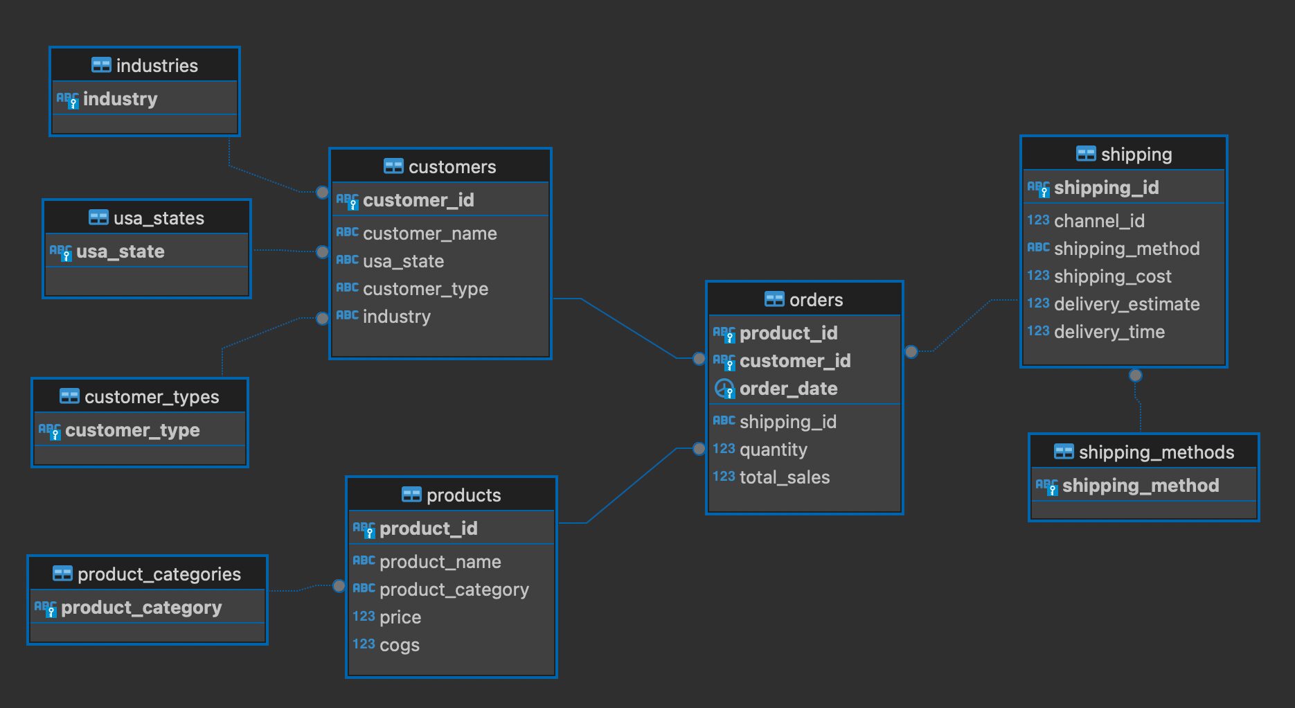
Database Schema

The relationships in the schema shows the relationships between the tables. All of these relationships are one-to-many. Often with orders and products there is a many-to-many relationship that requires an additional table, often referred to as a linking, association or bridge table. This is because an order can have many products and a product can be found in many orders. This is not the case with this data, where each order has only one product.
We could use the database to pull the data into R , but moving into the next step (analysis & visualization), it will be more efficient to use the data that we have already loaded. If this data was already in a database and the volume was exponentially larger, it would make sense to query the database first to limit the data, then load the data into R from there.
Data Analysis – Step 3: Data Analysis and Visualization
Now that we have cleaned & integrated the data, it’s time for data analysis & visualization. There are three areas that we are asked to analyze:
- Identify trends in sales performance across different product categories & customer types.
- Evaluate the efficiency of shipping methods & their impact on customer satisfaction.
- Assess the effectiveness of marketing spend by comparing the ROI across different industries.
IRL, I would want to know a lot more about each of these areas. It is always an important step to have discussions with stakeholders and understand the interests and concerns of those involved. I generally will have a meeting to understand the ask in more detail. Next, I would do an analysis and present what I have found. After that, there would likely be a round of updates to the analysis and another presentation. This could happen a few times. That is why creating reproducible analytics (code-based analysis) is so important. However, in this case, we’re going to make a number of assumptions and do the best we can.
To identify trends in sales performance across different product categories & customer types we have identified product categories (product_categories) and customer types (customer_types). From the orders table, we have identified sales (total_sales). It looks like we have what we need to fulfill the requested analysis.
For the second request, evaluate the efficiency of shipping methods & their impact on customer satisfaction, we have identified the shipping method (shipping_method) and it seems like we can use the estimated delivery time (delivery_estimate) and the actual delivery time (delivery_time) to evaluate the efficiency of shipping methods. However, we have no customer satisfaction data. IRL, I would ask for clarification on this one. What we’re going to do here is assume that the closer the delivery_time is to the delivery_estimate, the more efficient the shipping method and the more satisfied the customer is likely to be.
For the final request, assess the effectiveness of marketing spend by comparing the ROI across different industries, we’ll use the marketing_spend table. This was not integrated with the other tables since there is no relationship between them. We will calculate the ROI for the total marketing spend and then for each industry and compare them.
Sales Performance Trends Across Product Category & Customer Types.
We have yet to create any graphs! So let’s create our first graph by taking a look at sales over time. We are going to graph sales by week, because by day would be too many data points and by month would be too few:
total_sales <- scales::dollar(sum(orders$total_sales))

orders |>
  dplyr::mutate(week_date = floor_date(order_date, unit = 'week')) |>
  dplyr::group_by(week_date, ) |>
  dplyr::summarise(total_sales = sum(total_sales)) |>
  dplyr::ungroup() |>
  ggplot(aes(x = week_date, y = total_sales)) +
    geom_line() +
    scale_x_date(date_labels = "%b", date_breaks = "1 month") +
    geom_smooth(method = "lm", se = FALSE, color = "green") +
    scale_y_continuous(labels = dollar) +
    labs(title = 'Sales by Week',
         x = 'Week',
         y = 'Sales')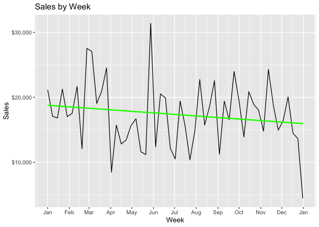
The total sales were \$920,589. We can see that the maximum sales were a little over \$30K during the last week of May, while the minimum sales was during the beginning of April (we’re not going to count the end of the year because that was not likely a full week). We have added a simple linear regression line in green. That smooths the sales numbers over time. We can see that it tilts slightly lower on the right than the left. That means that sales were decreasing over time.
Lets now look at sales by product category:
product_categories_totals <-
  orders |>
    dplyr::left_join(products, by = 'product_id') |>
    dplyr::group_by(product_category) |>
    dplyr::summarise(total_sales = sum(total_sales))

vapor_barrier <- product_categories_totals |>
                    dplyr::filter(product_category == 'vapor barrier') |>
                    dplyr::select(total_sales)
vapor_barrier <-  as.numeric(vapor_barrier$total_sales)
vapor_barrier <-  scales::dollar(vapor_barrier)

accessory <- product_categories_totals |>
                    dplyr::filter(product_category == 'accessory') |>
                    dplyr::select(total_sales)
accessory <-  as.numeric(accessory$total_sales)
accessory <-  scales::dollar(accessory)

orders |>
  dplyr::left_join(products, by = 'product_id') |>
  dplyr::mutate(week_date = floor_date(order_date, unit = 'week')) |>
  dplyr::group_by(week_date, product_category) |>
  dplyr::summarise(total_sales = sum(total_sales)) |>
  dplyr::ungroup() |>
  ggplot(aes(x = week_date, y = total_sales, color = product_category)) +
    geom_line() +
    scale_x_date(date_labels = "%b", date_breaks = "1 month") +
    geom_smooth(method = "lm", se = FALSE) +
    scale_y_continuous(labels = dollar) +
    labs(title = 'Product Category - Sales by Week',
         x = 'Week',
         y = 'Sales',
         color = 'Product Category')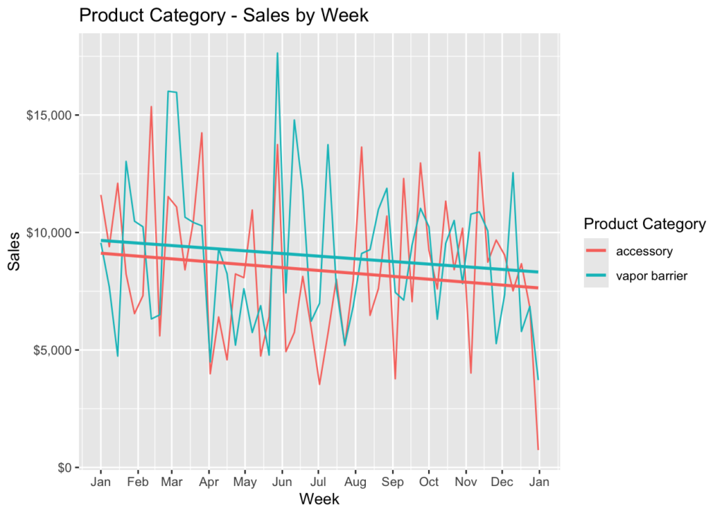
As you can see, the slope of the regression line is the same for both, in a negative direction. However, they each have different sales highs and lows. The highest was at the end of May for vapor barrier and the lowest was in the beginning of July for accessory. The total sales for vapor barrier was \$476,469 and \$444,120 for accessory.
Now let’s look at sale by customer type:
customer_type_totals <-
  orders |>
    dplyr::inner_join(customers, by = c('customer_id')) |>
    dplyr::group_by(customer_type) |>
    dplyr::summarise(total_sales = sum(total_sales))

distributor <- customer_type_totals |>
                    dplyr::filter(customer_type == 'distributor') |>
                    dplyr::select(total_sales)
distributor <-  as.numeric(distributor$total_sales)
distributor <-  scales::dollar(distributor)

ecommerce <- customer_type_totals |>
                    dplyr::filter(customer_type == 'e-commerce') |>
                    dplyr::select(total_sales)
ecommerce <-  as.numeric(ecommerce$total_sales)
ecommerce <-  scales::dollar(ecommerce)

orders |>
  dplyr::inner_join(customers, by = 'customer_id') |>
  dplyr::mutate(week_date = floor_date(order_date, unit = 'week')) |>
  dplyr::group_by(week_date, customer_type) |>
  dplyr::summarise(total_sales = sum(total_sales)) |>
  dplyr::ungroup() |>
  ggplot(aes(x = week_date, y = total_sales, color = customer_type)) +
    geom_line() +
    scale_x_date(date_labels = "%b", date_breaks = "1 month") +
    geom_smooth(method = "lm", se = FALSE) +
    scale_y_continuous(labels = dollar) +
    labs(title = 'Customer Type - Sales by Week',
         x = 'Week',
         y = 'Sales',
         color = 'Customer Type')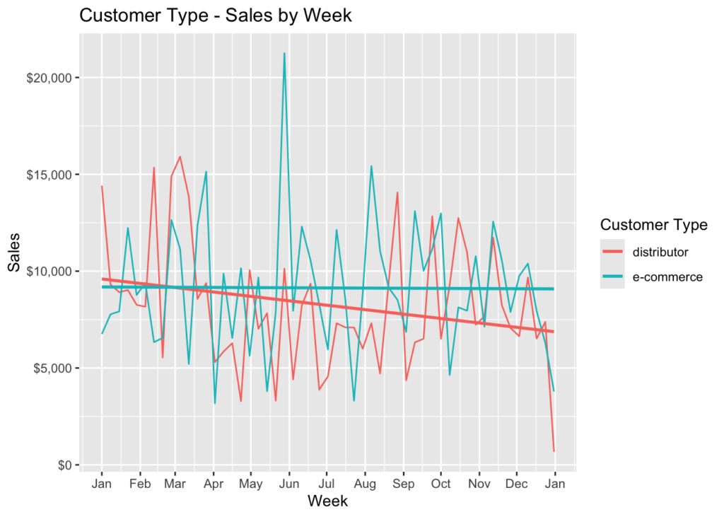
This is more interesting. Sales to distributors is sloping down, while sales to e-commerce customers is staying about even throughout the year. Also, there is a noticeable spike in the data for e-commerce sales. E-commerce sales were \$484,109 and distributor sales were \$436,480.
We can also take this chart and facet it by product category:
orders |>
  dplyr::inner_join(customers, by = 'customer_id') |>
  dplyr::left_join(products, by = 'product_id') |>
  dplyr::mutate(week_date = floor_date(order_date, unit = 'week')) |>
  dplyr::group_by(week_date, customer_type, product_category) |>
  dplyr::summarise(total_sales = sum(total_sales)) |>
  dplyr::ungroup() |>
  ggplot(aes(x = week_date, y = total_sales, color = customer_type)) +
    geom_line() +
    scale_x_date(date_labels = "%b", date_breaks = "1 month") +
    geom_smooth(method = "lm", se = FALSE) +
    scale_y_continuous(labels = dollar) +
    facet_wrap(~product_category, ncol = 1) +
    labs(title = 'Customer Type - Sales by Week',
         subtitle = 'Faceted by Product Category',
         x = 'Week',
         y = 'Sales',
         color = 'Customer Type')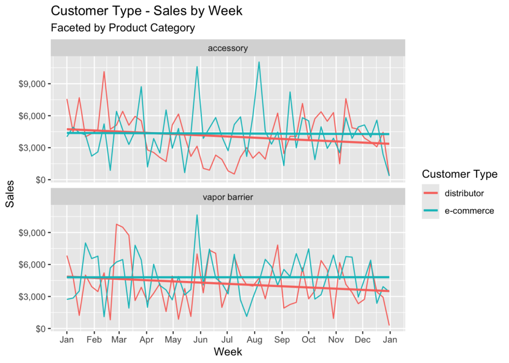
It appears that the trend is the same regardless of product category – distributor sales are down and e-commerce sales are flat.
Time-Series ARIMA Model
An ARIMA model is used in data analysis to predict future values and works best with at least a few years of data. However, we will go through the steps in creating one and check the results. We’ll do this for the total sales by week. If you are unfamiliar with ARIMA models, I wrote an introduction (https://rebrand.ly/l1tf4p1).
First we need to create a time-series object from a dataframe and plot the results:
sales_by_week <-
  orders |>
    dplyr::mutate(week_date = floor_date(order_date, unit = 'week')) |>
    dplyr::group_by(week_date, ) |>
    dplyr::summarise(total_sales = sum(total_sales)) |>
    dplyr::ungroup()

# There are 53 periods from start = 1/1/2023 to end = 12/31/2023 (by week).
# We need to get the start and end dates.
start_date <- as.Date(min(sales_by_week$week_date))
end_date <- as.Date(max(sales_by_week$week_date))

# Creating the time-series object.
# Frequecy is the number of periods in a cycle.
# I'm going to use 4 (each cycle is a month)
# because we only have a year's worth of data.
sales_data_ts <- ts(sales_by_week$total_sales,
                    start = c(year(start_date), week(start_date)),
                    end = c(year(end_date), week(end_date)), frequency = 4)

plot(sales_data_ts, xlab = "Week", ylab = "Sales")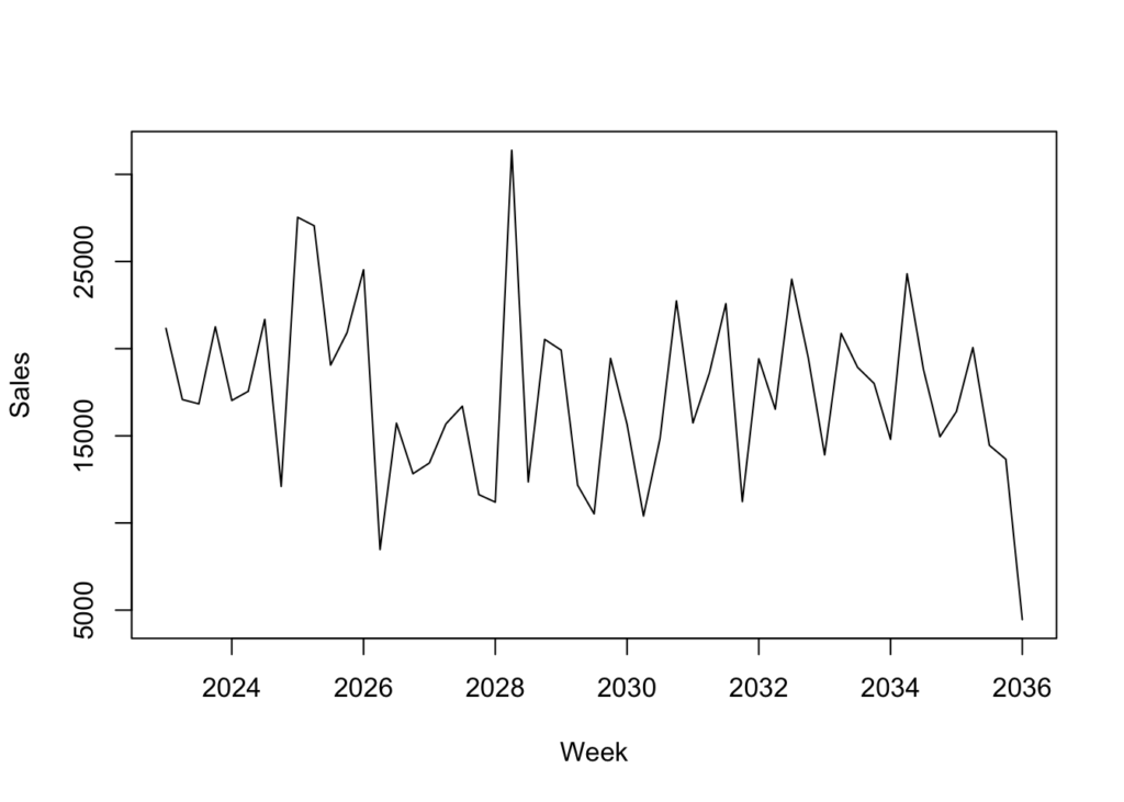
We don’t see any real trending so we’ll use an augmented Dickey-Fuller test to determine if the dataset is stationary & we’ll decompose the data into its components:
library(urca)

# Augmented Dickey-Fuller test.
summary(ur.df(sales_data_ts, type = 'trend', lags = 4))
###############################################
# Augmented Dickey-Fuller Test Unit Root Test #
###############################################

Test regression trend


Call:
lm(formula = z.diff ~ z.lag.1 + 1 + tt + z.diff.lag)

Residuals:
     Min       1Q   Median       3Q      Max
-12689.4  -3336.7    196.2   2882.3  13032.3

Coefficients:
              Estimate Std. Error t value Pr(>|t|)
(Intercept)  1.848e+04  6.720e+03   2.751  0.00881 **
z.lag.1     -9.804e-01  3.590e-01  -2.731  0.00926 **
tt          -5.601e+01  5.547e+01  -1.010  0.31859
z.diff.lag1 -7.486e-02  3.333e-01  -0.225  0.82344
z.diff.lag2  1.982e-03  3.053e-01   0.006  0.99485
z.diff.lag3  2.458e-01  2.465e-01   0.997  0.32469
z.diff.lag4  2.452e-01  1.647e-01   1.488  0.14434
---
Signif. codes:  0 '***' 0.001 '**' 0.01 '*' 0.05 '.' 0.1 ' ' 1

Residual standard error: 5297 on 41 degrees of freedom
Multiple R-squared:  0.5564,    Adjusted R-squared:  0.4915
F-statistic: 8.573 on 6 and 41 DF,  p-value: 4.666e-06


Value of test-statistic is: -2.7312 2.7731 4.011

Critical values for test statistics:
      1pct  5pct 10pct
tau3 -4.04 -3.45 -3.15
phi2  6.50  4.88  4.16
phi3  8.73  6.49  5.47
# We're going to use additive decomposition because
# we can see that the magnitude of seasonality
# is relatively constant over time,
sales_data_decomp <- decompose(sales_data_ts, type = 'additive')
plot(sales_data_decomp, xlab = 'Week')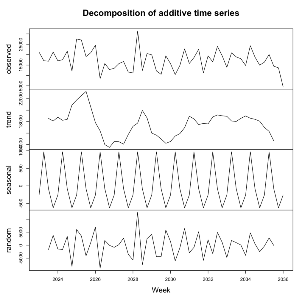
We can tell from the difference between the test-statistic and tau3 that the data is not stationary. We can also see that there is regular seasonality (this is over monthly periods) that appears a little too perfect. There is also a slight trend downward and some random noise as well.
Let’s look at the ACF & PACF – these check which lags are significant by identifying the relationship between observations at different lags:
forecast::tsdisplay(sales_data_ts) 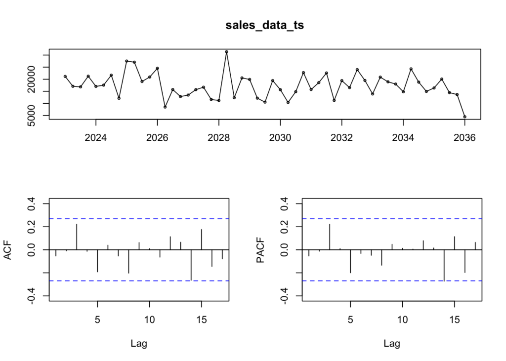
Because none of the vertical lines cross the horizontal lines in either the ACF or PACF, there are no relevant lags in the data. This means that we cannot predict future trending based on the data we have so far. We would need to either wait for more data to be collected or add data from further in the past to be able to make future predictions.
Summary
The story that is emerging from this data analysis is that distributor sales are declining while e-commerce sales are flat. They are very close, in terms of sales, with e-commerce making up 53% of sales and distributor sales making up 47%. However, if this trend continues, e-commerce customers will become increasingly important, while distributors will be less so.
We should recommend investigating why distributor sales are declining. We should also focus on understanding why e-commerce sales have been flat. If this is an ongoing trend, it might be worth it to spend more time on growing e-commerce sales, unless there is a solution to declining distributor sales. Understanding more about the business is critical to understanding these trends and having more data can help in predicting future sales behavior.
Overall, both product categories make up a similar amount of the business, with vapor barrier making up 52% of sales and accessory making up 48% of sales. Both are declining and this is due to distributor sales. Sales for both product categories are flat for e-commerce sales.
Efficiency of Shipping Methods & Customer Satisfaction Impact
To understand the efficiency of shipping methods, as well as customer satisfaction, we are going to compare the estimated time of delivery to the actual delivery time by shipping method. We are going to subtract the delivery_time from the delivery_estimate, so that if a delivery were estimated to be delivered at 7, but was actually delivered at 8, we would subtract 8 from 7 for a difference of -1. We will assume that a zero is average, a negative value is less efficient and a positive value is more efficient.
The first thing we want to understand is the average cost of each shipping method. To do that, we are going to create a table with each shipping method and the average cost:
shipping_methods_cost <-
  shipping |>
        dplyr::group_by(shipping_method) |>
        dplyr::summarise(shipping_cost = dollar(mean(shipping_cost))) |>
        dplyr::rename(`Shipping Method` = shipping_method,
                      `Avg. Shipping Cost` = shipping_cost)

knitr::kable(shipping_methods_cost)| Shipping Method | Avg. Shipping Cost |
|---|---|
| Express | $27.98 |
| Overnight | $27.10 |
| Standard | $27.12 |
There is not much difference in cost between different shipping methods. Personally, I think I would always choose Overnight, unless Express is even faster. I suspect that Standard would be the slowest. Next, let’s check the average difference between the estimated delivery time and the actual delivery time by shipping method:
shipping_methods_diff <-
  shipping |>
      dplyr::mutate(shipping_days_diff = delivery_estimate - delivery_time) |>
      dplyr::group_by(shipping_method) |>
      dplyr::summarise(shipping_days_diff = round(mean(shipping_days_diff), 3)) |>
      dplyr::rename(`Shipping Method` = shipping_method,
                    `Avg. Shipping Diff` = shipping_days_diff)

knitr::kable(shipping_methods_diff)| Shipping Method | Avg. Shipping Diff |
|---|---|
| Express | -0.003 |
| Overnight | 0.033 |
| Standard | -0.015 |
On average, Overnight appears to be the most efficient shipping method. Standard appears to be the least, with Express in the middle. Let’s look at efficiency over time as well to see if there are any variations:
shipping |>
  dplyr::inner_join(orders, by = 'shipping_id') |>
  dplyr::mutate(shipping_days_diff = delivery_estimate - delivery_time,
                week_date = floor_date(order_date, unit = 'week')) |>
  dplyr::group_by(shipping_method, week_date) |>
  dplyr::summarise(shipping_days_diff = round(mean(shipping_days_diff), 3)) |>
  ggplot(aes(x = week_date, y = shipping_days_diff, color = shipping_method)) +
    geom_line() +
    scale_x_date(date_labels = "%b", date_breaks = "1 month") +
    geom_smooth(method = "lm", se = FALSE) +
    #scale_y_continuous(labels = dollar) +
    labs(title = 'Shipping Method - Sales by Week',
         x = 'Week',
         y = 'Avg. Est. Diff.',
         color = 'Shipping Method')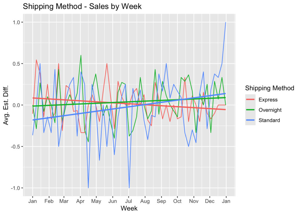
It looks like the Standard shipping method has improved in efficiency over time, while Express has declined, with a slight improvement for Overnight. With its declining efficiency, I think I might change my mind and choose Standard for greater satisfaction (particularly toward the end of the year). However, some of the greatest negative spikes comes from Standard shipping and only at the end of the year did it really improve its efficiency.
Summary
We made the assumption that greater efficiency was defined by a lesser value of delivery_time compared to delivery_estimate, which would indicate that the delivery was either on time or earlier than expected. We also assumed that receiving a delivery on time would be satisfactory and that the earlier the delivery arrived compared to expected, the greater the customer satisfaction.
Overnight had the best average efficiency, therefore the best average customer satisfaction. It was consistant throughout the year.
Express was in the middle in terms of efficiency, so we concluded that the average customer satisfaction was in the middle. However, the efficiency declined throughout the year, so it is likely that customer satisfaction also declined.
Standard improved dramatically toward the end of the year. It started the year with the lowest efficiency, but ended with the highest. We would conclude the same for customer satisfaction.
We should recommend reviewing Express and understanding why the efficiency slid during the year and what can be done to improve it. We should also review Standard to understand the reasons behind how it improved as it did. Those reason might be able to be applied to Express.
Marketing Spend Effectiveness – ROI Comparison Across Industries
The return on investment for marketing spend is often called return on ad spend or ROAS. One of the issues that I have had with ROAS is that it can never be negative:
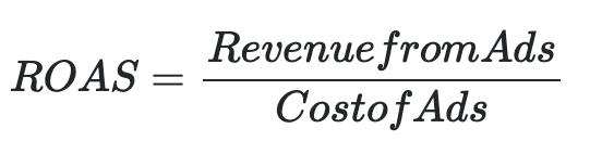
If you lost half of your investment, your ROAS would be 50% or 0.5. On the other hand, ROI would be -50% or -0.5:
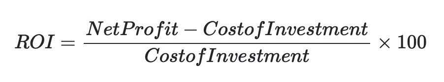
Let’s use ROI for this analysis and calculate the ROI of our total marketing spend and then by industry and compare:
total_marketing_spend <- sum(marketing_spend$marketing_spend)
total_revenue <- sum(marketing_spend$revenue)

total_roi <- ((total_revenue -
               total_marketing_spend) /
               total_marketing_spend)
In total, \$117,831 was spent on marketing. We can credit \$643,246 in revenue to the marketing dollars spent. That gives us an ROI of 446%. Another way to state this is that for every 1 dollar of marketing spent, 4.46 dollars are returned as revenue.
Now let’s look at the ROI by industry:
marketing_spend |>
  dplyr::mutate(ROI = round(((revenue -
               marketing_spend) /
               marketing_spend), 2)) |>
  dplyr::mutate(`Marketing Spend` = scales::dollar(marketing_spend),
                Revenue = scales::dollar(revenue),
                Industry = industry) |>
  dplyr::select(Industry,
                `Marketing Spend`,
                Revenue,
                ROI) |>
knitr::kable()| Industry | Marketing Spend | Revenue | ROI |
|---|---|---|---|
| commercial | $36,548.03 | $339,241 | 8.28 |
| residential | $81,282.90 | $304,006 | 2.74 |
The ROI from commercial marketing is far higher than the the ROI from residential. However, for each industry, the ROI is positive and is not wasted.
Summary
The overall ROI is very strong and positively contributes to revenue. Commercial marketing spend is far more effective, with an ROI of 8.28 or 828%. That does not mean that residential marketing spend is not effective. Residential revenue was nearly 3x the marketing spend. It only means that commercial marketing spend was more effective. There could be a number of reasons for this. It could be the difference in the industries or the marketing tactics used or the channels available to each industry. It would be interesting to view this data as a trend over time to see if there are more effective times to spend on marketing than other times.
Conclusion
We have completed all the objectives of this data analysis. First, we analyzed the datasets by uploading them as data frames and reviewing each of them to understand the data they contain. We drew some conclusions and made a few updates to the data and metadata. Next, we modeled this data in a database, created the primary keys and foreign key constraints. We added a few auxiliary tables to better define certain attributes. Then we laid out the data schema. Finally, we analyzed sales trends, attempted to build an ARIMA model, analyzed shipping efficiency and customer satisfaction and calculated total marketing ROI and the marketing ROI by industry and analyzed the results.
I hope you have found this insightful and maybe has given you some ideas for your own end-to-end analytics tasks. If you have never worked with R or another analytical programming language, I hope this provides you with some understanding of the power of reproducible analytics.